RAnEnExtra::subsetCoordinates

RAnEnExtra::subsetCoordinates extracts the coordinates within an predefined extent or the coordinates that are closest to a set of target coordinates based on Eucleadian distances. This function can also write the corresponding IDs to the extracted coordinates into a file so that it can be used in other executables provided in the PAnEn packages.

subsetCoordinates(
  xs,
  ys,
  poi,
  file.output = NULL,
  arg.name = "stations-index",
  num.chunks = NULL,
  num.cores = 1
)

Arguments

xs	A vector with X coordinates.
ys	A vector with Y coordinates.
poi	Points of interest, or target points. It can be either a named vector with left, right, top, and bottom or a data frame for a set of target point coordinates as rows with variable names X and Y.
file.output	A file name to write the ID of subset stations.
arg.name	The configuration argument name. By default, it is stations-index from anen_grib and grib_convert.
num.chunks	How many chunks to break the stations into. Each chunk will be saved to a separate configuration file.
num.cores	Set this to the number of paralell cores to use. Default to 1.

Value

A data frame with ID and coordinates for subset stations. The column ID.C should be used for C++ programs. The column ID.R should be used in R.

Examples

####################################################################
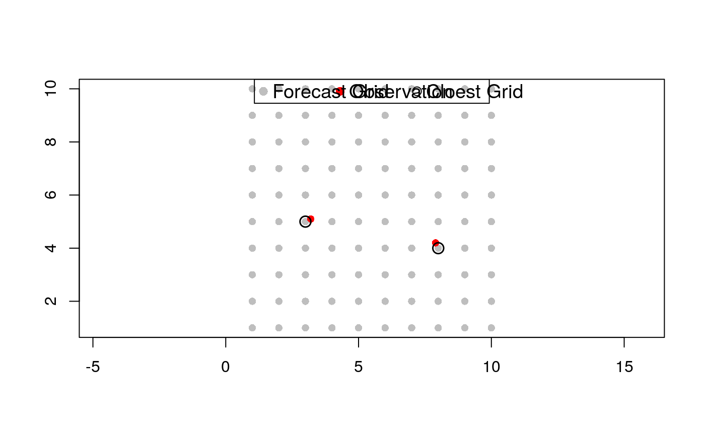
#                       Use Case 1                                 #
####################################################################

# Define the forecast grid coordinates
forecast.grids <- expand.grid(X = 1:10, Y = 1:10)

# Define the observation coordinates
obs.coords <- data.frame(X = c(3.2, 7.9), Y = c(5.1, 4.2))

# Find the closest forecast grid to each observation location
subset.coords <- subsetCoordinates(
  forecast.grids$X, forecast.grids$Y, obs.coords)

# Visualization
plot(forecast.grids$X, forecast.grids$Y, pch = 16,
     cex = 1, col = 'grey', asp = 1, xlab = '', ylab = '')
points(obs.coords$X, obs.coords$Y, pch = 16, cex = 1, col = 'red')
points(subset.coords$X, subset.coords$Y, cex = 1.5, lwd = 1.5)
legend('top', legend = c('Forecast Grid', 'Observation', 'Cloest Grid'),
       col = c('grey', 'red', 'black'), pch = c(16, 16, 1),
       horiz = T, cex = 1.2)

####################################################################
#                       Use Case 2                                 #
####################################################################

# Define a region of interest
extent <- c('left' = 2.5, 'right' = 8,
            'top' = 8.9, 'bottom' = 2)

# Subset the forecast grids within the extent
subset.coords <- subsetCoordinates(
  forecast.grids$X, forecast.grids$Y, extent)

# Visualization
plot(forecast.grids$X, forecast.grids$Y, pch = 16,
     cex = 1, col = 'grey', asp = 1, xlab = '', ylab = '')
rect(xleft = extent['left'], xright = extent['right'],
     ybottom = extent['bottom'], ytop = extent['top'],
     cex = 1, col = NA, lwd = 1, lty = 'dashed')
points(subset.coords$X, subset.coords$Y, cex = 1.5, lwd = 1.5)
legend('top', legend = c('Forecast Grid', 'Subset Grid'),
       col = c('grey', 'black'), pch = c(16, 1),
       horiz = T, cex = 1.2)